Time-resolved photoluminescence alone does not fix a carrier lifetime
Fitting exponentials to a time-resolved photoluminescence decay to extract a carrier lifetime is the basic procedure in evaluating an emissive material. A Sungkyunkwan University group has demonstrated that the value is not uniquely determined. Entirely different coefficient sets produce almost identical decay curves. Measuring photoluminescence quantum yield alongside separates them, and deep learning resolves all six coefficients at once.
This article was published before the English edition began, so the labels inside its figures and simulators are in Korean. The caption and the note under each figure are in English.
DOI 10.1038/s41467-026-77052-8One of the first measurements made when evaluating an emissive material is time-resolved photoluminescence (TrPL). You hit the sample with a light pulse, record the curve as the light dies away, and fit exponentials to it to extract a carrier lifetime. That is the number written in papers and reports as “a lifetime of so many nanoseconds.”
What the Sungkyunkwan University group has now confirmed is this. That number is not uniquely determined.
Six recombination coefficients can be combined in entirely different ways and still produce decay curves that almost completely overlap. Zooming in on two such cases in simulation, they were indistinguishable within realistic measurement noise. Since the curves are the same, the lifetime extracted by fitting comes out the same as well, but the physics actually taking place inside is different.
The group solved this by measuring photoluminescence quantum yield (PLQY) alongside. They then built and released a deep-learning model that extracts all six coefficients at once when both datasets are supplied.
1. The ambiguity of a number called lifetime
Fitting exponentials to a TrPL decay is convenient. The problem is that this approach lumps several intertwined pathways inside perovskite and other semiconductors into a single exponential term. On top of that, the lifetime so obtained varies greatly with measurement conditions. The paper is blunt about it: a lifetime extracted this way may not carry a clear physical interpretation.
The differential decay time used as an alternative is no better off. Plotting it as a function of time hides quantitative kinetic information, because the effective bimolecular recombination coefficient is not conserved. Information such as recombination mediated by shallow traps disappears in the process.
Doing it properly in physical terms means setting up rate equations, solving simultaneously for the time evolution of electrons, holes and trapped electrons. Two walls stand here as well.
First, the model has to be fixed in advance from limited observations. Second, the several recombination pathways are strongly entangled, so the same TrPL decay is reproduced by several different coefficient sets. That is the multiple-solution problem this paper takes on head-on.
2. Overlapping curves
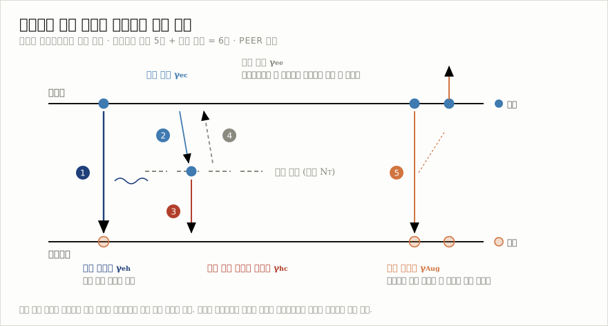
The model the group set up holds five pathways.
| No. | Pathway | Coefficient |
|---|---|---|
| ① | direct recombination of conduction band electrons and valence band holes | γeh |
| ② | capture of an electron by a trap | γec |
| ③ | non-radiative recombination of a trapped electron with a hole | γhc |
| ④ | re-emission of a trapped electron | γee |
| ⑤ | Auger recombination | γAug |
Adding the trap density NT makes six unknowns. Because the exciton binding energy in perovskite is comparable to room-temperature thermal energy, excitons are taken to dissociate quickly and are left out of the calculation.
Varying the coefficients and plotting decay curves, the shapes diverged as expected. But for certain pairs of sets the curves folded into what was effectively one line. Even magnified, the difference was smaller than realistic measurement noise.
This is where the group brought in photoluminescence quantum yield. It is the ratio of photons emitted to photons absorbed, and measuring it while varying excitation intensity gives a curve.
For those two cases whose TrPL curves overlapped, the quantum yield curves separated clearly.
The reason lies in the definition of quantum yield. Through the charge neutrality condition, the value is sensitive to how far the traps are filled. It is not a matter of adding more data points; it places a constraint of a different character on the steady-state carrier distribution and on the split between radiative and non-radiative pathways.
Moving the coefficients one at a time makes that complementarity clearer still.
| Coefficient | In TrPL | In quantum yield |
|---|---|---|
| trap density NT | weak variation in the low region | clear even in the low region |
| electron emission γee | barely visible over two orders of magnitude | distinguishable in the low generation rate range |
| Auger γAug | small influence | lowers the peak at high generation rates |
The electron emission coefficient in particular is an important value governing long-time behaviour, and yet a difference of two orders of magnitude did not stand out in TrPL alone.
Below is a direct solution of the paper’s rate equations. Move the coefficients with the sliders and the decay curve on the left barely stirs while the quantum yield curve on the right clearly separates. Pushing the electron emission coefficient across its full two orders of magnitude makes the difference plainest.
3. Why deep learning was attached
Adding one more constraint does not by itself hand over the six coefficients. Iterative optimization has to be run for every new sample, and local minima can be fallen into again along the way.
The group chose instead to train on large-scale simulated data generated from the physical model. They drew the six coefficients and the initial carrier density at random within physically sensible ranges to make 200,000 sets, and computed a TrPL and a quantum yield curve for each as the paired target.
| Item | Value |
|---|---|
| Training set | 200,000 |
| Input | TrPL 200 points + quantum yield 200 points + initial carrier density = 401 |
| Network | 401 : 1800 : 1800 : 6, dropout 0.048 |
| Implementation | PyTorch (Python 3.12.7) |
| Release | database, trained model and code all public |
The advantage of this arrangement is that once trained, coefficients come straight out on feeding in new measurement data.
4. What you put in decides the result
The table that says the most in this paper is the one below. It is the same network trained with only the input changed.
| Training input | γeh | γec | γhc | NT | γee | γAug |
|---|---|---|---|---|---|---|
| TrPL alone | 0.86 | 0.31 | 0.50 | 0.74 | 0.38 | 0.057 |
| quantum yield alone | 0.75 | 0.66 | 0.64 | 0.74 | 0.64 | 0.83 |
| TrPL + quantum yield | 0.92 | 0.80 | 0.76 | 0.92 | 0.83 | 0.94 |
| after optimization | 0.996 | 0.938 | 0.969 | 0.988 | 0.905 | 0.973 |
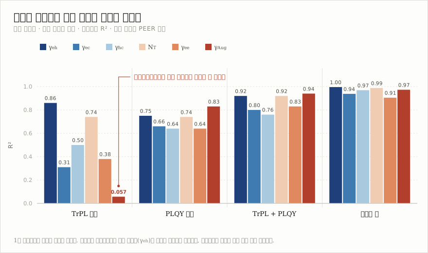
These are coefficients of determination. The closer to 1, the closer the prediction to the truth.
With TrPL alone the coefficient of determination for Auger recombination stops at 0.057. That means essentially nothing can be extracted. Only the direct recombination coefficient holds up at 0.86, while electron capture falls to 0.31 and electron emission to 0.38.
Quantum yield alone is not enough either, because it is a steady-state value and cannot account for instantaneous changes in emission. Only with both datasets together do all six come alive.
Real measurements carry noise, so that condition was checked too. Trained on data with noise deliberately mixed in, only the electron emission coefficient fell, to 0.73, while the rest held above 0.84.
5. On real samples
To show this is not confined to simulated data, four perovskite films were made and measured: two compositions (FAMA, CsFAMA), each with and without a 4-MeO-PEAI surface treatment.
| Sample | Grain size | Bandgap |
|---|---|---|
| FAMA | 962±302nm | 1.567 eV |
| FAMA + passivation | 1.573 eV | |
| CsFAMA | 682±227nm | 1.571 eV |
| CsFAMA + passivation | 1.577 eV |
Film thickness is about 500nm. Coefficients obtained by fitting the measured curves with a genetic algorithm were placed alongside those the deep-learning model predicted, and the two agreed well. The error of the fit itself ran between a mean squared error of 2.72×10⁻⁵ and 1.12×10⁻⁴ in TrPL.
How the coefficients moved before and after passivation is the part especially worth watching.
| Coefficient | FAMA | CsFAMA |
|---|---|---|
| direct recombination γeh | 2.72 → 3.61 (×10-11 cm3/s) | 1.87 → 2.65 (×10-11 cm3/s) |
| trap density NT | 7.31 → 4.88 (×1015 cm-3) | 7.35 → 6.05 (×1015 cm-3) |
The radiative coefficient went up and the trap density went down. What the surface treatment did is split out in numbers. The electron capture and hole capture coefficients fell as well.
Devices were then built from the same films for comparison: n-i-p structure solar cells.
| Sample | Conversion efficiency | Ideality factor |
|---|---|---|
| FAMA | 22.41% | 1.42 kBT/q |
| FAMA + passivation | 25.08% | 1.18 kBT/q |
| CsFAMA | 21.64% | 1.38 kBT/q |
| CsFAMA + passivation | 23.23% | 1.16 kBT/q |
An ideality factor moving toward 1 means trap-mediated recombination has fallen, and impedance measurements likewise showed the recombination resistance growing. The direction predicted optically and the direction measured electrically were the same.
6. A proposal on measurement conditions
There is one more item in this paper that a practitioner can use straight away.
How long to record TrPL for, and where to cut off the decay, differ from study to study. With no standard, reported lifetimes end up being values that depend on the measurement window and fitting method rather than intrinsic properties of the material.
The group trained the model while varying the time window and cutoff to find a criterion.
| Item | Recommendation |
|---|---|
| Acquisition time window | 2μs |
| Decay cutoff | 0.01 |
| Range of application | initial carrier density 1015 to 1017 cm-3 |
| Corresponding excitation | 100 to 2000 nJ/cm2 |
Under these conditions more than 95% of the area under the decay curve is preserved. Narrowing further degraded prediction accuracy noticeably. They also state that this criterion does not carry over to every material. For high-quality single crystals, two-dimensional perovskites and nanocrystals, their recommendation is to train a model of one’s own by the same methodology.
7. What it means
The device validation in this paper was done with solar cells. But the multiple-solution problem itself bears more directly on those working with light-emitting devices.
Measuring a carrier lifetime by TrPL and comparing materials by that value is a procedure repeated as is in evaluating OLED, quantum dot and micro-LED materials. The paper itself cites OLED work as a starting point: earlier research that used deep learning on time-resolved electroluminescence to extract polaron recombination and triplet-triplet annihilation coefficients. That approach yields only one coefficient at a time, which this paper marks as the point to get past.
Three things remain.
First, a condition now attaches to the practice of comparing materials by a single lifetime. If the same lifetime can arise from different physics, then two materials having the same lifetime is not on its own enough to call them the same. Conversely, when lifetimes differ, that number alone does not say which pathway changed.
Second, the demand to measure quantum yield as a function of excitation intensity can be met without extra equipment. Anywhere with an integrating sphere and a spectrometer already makes this measurement; what is added is the labour of taking several points while varying the excitation. In return, six coefficients come apart.
Third, it connects to the other article in this issue. The germanium exciplex host study introduced on the same day rests its argument on a delayed fluorescence lifetime falling from 1.9μs to 1.6μs. What conditions make such a lifetime a trustworthy number is exactly what this paper deals with. Research that makes a material and research that sharpens how the material is measured appeared side by side in the same week.
Worth adding is that the database, the trained model and the code are all public. Anyone wanting to retrain a model for their own material does not have to build one from scratch.
Sources
- Chen, W., Ahn, H. C., Jo, B. et al. Resolving carrier kinetics in perovskite through deep-learning-assisted photoluminescence analysis. Nature Communications (2026). Published online 2026-08-21. DOI 10.1038/s41467-026-77052-8 · CC BY-NC-ND 4.0
- Every figure in the text is a value confirmed directly in the body, tables and figure captions of that paper. Values from samples of different composition were not mixed into a single row.
- The paper is released under CC BY-NC-ND 4.0, so its original figures are not reproduced here. The two figures in the text were newly drawn by this magazine from the model and values the paper presents.